WARDEN

Authors	Lance Palmer, Andrew Frantz
Publication	N/A (not published)
Technical Support	Contact Us

Overview

The WARDEN (Workflow for the Analysis of RNA-Seq Differential ExpressioN) software uses RNA-Seq sequence files to perform alignment, coverage analysis, feature counts and differential expression analysis.

There are 3 entrypoints to the WARDEN workflow. The start-to-end workflow begins with FASTQ files which are aligned by STAR. WARDEN can optionally be entered at this point with user-aligned RNA-Seq BAMs. Aligned BAMs are then run through HTSeq-count to determine the number of reads mapping to features. The next stage can also be entered with user-derived count files, where differential expression analysis is performed on the defined cohorts.

Workflow Steps

1. FASTQ files generated by RNA-Seq are mapped to a reference genome using the STAR.
2. HTSeq-count is used to assign mapped reads to features (default feature is gene).
3. Differential expression analysis is performed using VOOM normalization of counts and LIMMA analysis.
4. Coverage plots of mapped reads are optionally generated as interactive visualizations.

Outputs

Name	Description
VOOM/LIMMA results and visualizations	Pairwise comparisons of expression data. Requires at least 3 samples vs 3 samples.
Simple Differential Expresssion results and visualizations	No advanced statistical analysis, requires only a 1 sample vs 1 sample comparison.
Feature counts	Feature counts generated by HT-Seq count.
FPKM values (optional)	If feature selection for HT-Seq count is genes, FPKM and FPKM-log2 values are calculated.
Aligned BAMs	Aligned BAM files from STAR mapping.
Splice junctions	Splice junction information from STAR mapping.
GSEA analysis inputs	Input files for more advanced GSEA analysis of the comparisons run.
Coverage files (optional)	bigWig (.bw) files detailing coverage. (Enabled via run_coverage option).
FastQC Reports (optional)	Quality control analysis by FastQC. (Enabled via run_FastQC option).

Inputs

Depending on which entry point is chosen, inputs may include an array of FASTQ files, RNA-Seq BAM files, or feature count files. All 3 entry points require a similarly formatted “sample sheet” which describes the relationships between samples.

Each WARDEN workflow requires an array of input files, a sample sheet, and has one to three parameters which must be set explicitly. All other parameters are preset with reasonable defaults.

Required Input	Description	Example
FASTQ files (WARDEN [FASTQ])	FASTQ files generated by RNA-Seq experiment	Sample1.fastq.gz, Sample2.fastq.gz
BAM files (WARDEN [BAM])	BAM files generated by RNA-Seq experiment	Sample1.bam, Sample2.bam
Count files (WARDEN [Counts])	Feature count files generated by RNA-Seq experiment. Must have a header line.	Sample1.htseq_counts.txt, Sample2.htseq_counts.txt
Sample sheet (all apps)	Sample sheet generated and uploaded by the user	Samplesheet.txt or Samplesheet.xlsx
Genome Build (all apps)	Which genome build to use for alignment and analysis	Human_hg38_v31, Mouse_mm10_v24, etc.
Sequencing Strandedness (WARDEN [FASTQ] and WARDEN [BAM])	Experimental procedure during sequencing	Unstranded, First strand synthesis, or Second strand synthesis
BAM sort order (WARDEN [BAM])	BAM file sort order	Name or Position

Sample sheet configuration

You’ll need to create a sample sheet which describes the relationship between case and control samples, phenotype/condition information, and the comparisons you would like to perform. The sample sheet is a white-space delimited text document that can be created in Microsoft Excel or a text editor. This file must have a header row labelling each column, though the names of the columns are up to the user. No names or fields are allowed to have white space characters (space, tab, etc.).

Using Microsoft Excel

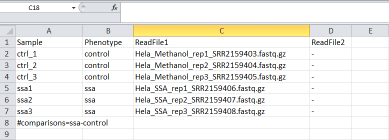
The final product for the excel spreadsheet will look like the screenshot below. If you create the sample sheet from scratch, please ensure the the columns are in this order.

Sample rows

Each row in the spreadsheet (except for the last row, which we will talk about in the next section) corresponds to a sample with one or more input files. You should fill in these rows based on your data and the guidelines below:

Comparison row

The last line in the sample sheet is called the “comparison row”. This line specifies the comparisons to be done between conditions/phenotypes. All pairwise combinations of the values in the “Phenotype” column can be analyzed. To specify the comparisons, on a separate line, include #comparisons= followed be a comma delimited list of two conditions/phenotypes separated by a dash. This line may appear anywhere in the file, but the examples place it at the bottom. There should not be white space between any of these characters.

Finalizing the sample sheet

To finalize the sample sheet, save the Microsoft Excel file with whatever name you like. Save the file as an Excel Workbook with the .xlsx extension.

Using a text editor

Creating a sample sheet with a text editor is another option. The process of creating a sample sheet with a text editor is the same as creating one with Microsoft Excel, with the small difference that you must create your columns using white-space (spaces or tabs). Save the file with a .txt extension.

Feature counts file format

WARDEN [Counts] needs feature count files to have a header that can link the files to the information in the sample sheet.

Each counts file should have a header with 2 tab seperated entries. The first is a label for the features, typically gene_name, but as long as it’s the same in each file the exact name doesn’t make a difference. The second column must be labelled with a sample name that appears in the “sample sheet”. Because of this linkage, WARDEN [Counts] will not attempt to correct malformed sample names in the sample sheet, but instead fail and ask you to manually conform to the requirements.

After the header, WARDEN expects a similar format to that output by HTSeq-count. In short, each row has a feature identifier followed by an integer count number, seperated by a tab.

Example:

gene_name ctrl_1
A1BG      10
A1BG-AS1  0
A1CF      4
A2M       477
...

Creating a workspace

Before you can run one of our workflows, you must first create a workspace in DNAnexus for the run. Refer to the general workflow guide to learn how to create a DNAnexus workspace for each workflow run.

You can navigate to the WARDEN Differential Expression Analysis workflow page here.

Uploading Input Files

The WARDEN Differential Expression analysis pipeline takes FASTQ files, BAM files, or feature count files generated by an RNA-Seq experiment as input.

Due to the dynamic nature of the WARDEN workflow, we recommend limiting the cohort in a single run to around 60 samples. Running with additional samples may lead to intermittent failures, especially when starting with FASTQs or BAMs.

Refer to the general workflow guide to learn how to upload input files to the workspace you just created.

Running the Workflow

Refer to the general workflow guide to learn how to launch the workflow, hook up input files, adjust parameters, start a run, and monitor run progress.

Hooking up Inputs

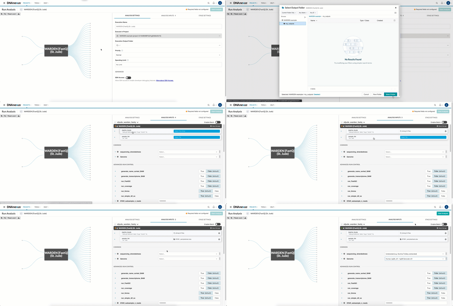
First, in the Execution Output Folder field, select a folder to output results in. You can structure your experiments however you like (e.g. /my_outputs). If left blank, a directory named with the execution ID will be created in order to avoid cluttering your workspace and keep seperate runs seperate.

Next, you’ll need to hook up the FASTQ files, BAM files, or count files (depending on which entrypoint you wish to use) and sample sheet you uploaded in the upload data section. Click the FASTQ_FILES, BAM_FILES, or COUNT_FILES input field and select all input files listed in your sample sheet. Next, click the sample_list input field and select the corresponding sample sheet.

If running “WARDEN [FASTQ]” or “WARDEN [BAM]”, select the sequence_strandedness drop down menu and choose the appropriate option. This information can be determined from the sequencing or source of the data. If you don’t know what to put here, select “Unstranded”.

If running “WARDEN [BAM]”, select the sort_order drop down menu and choose the method with which your BAM files are sorted, either name or position. Unsorted BAM files are not supported by WARDEN.

Finally, select the Genome pulldown menu, choose the appropriate option, and WARDEN is ready to be run! For “WARDEN [FASTQ]“, Genome determines which genome STAR will map your FASTQs to. For “WARDEN [BAM]” and “WARDEN [Counts]“, Genome should be which genome your BAM files or counts files were previously aligned to.

Continue reading to learn about the available advanced options.

Selecting Parameters

For the general workflow instructions on parameter selection, refer here.

Once all parameters have been adjusted to your needs, you’re ready to run WARDEN!

Summary of Results

Each tool in St. Jude Cloud produces a visualization that makes understanding results more accessible than working with excel spreadsheet or tab delimited files. This is the primary way we recommend you work with your results.

Refer to the general workflow guide to learn how to access these visualizations.

We also include the raw output files for you to dig into if the visualization is not sufficient to answer your research question.

Refer to the general workflow guide to learn how to access raw results files.

Primary Results

Multidimensional scaling (MDS) Plot

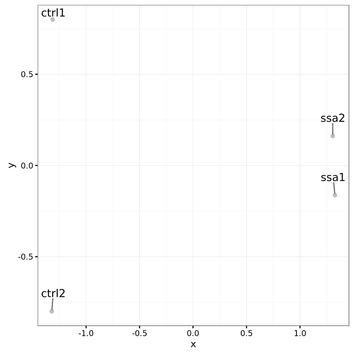
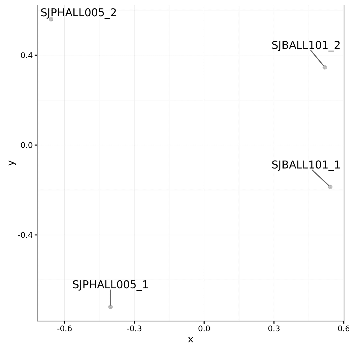
Multidimensional scaling (MDS) plots are created using the plotMDS function within LIMMA. Similar to PCA, these graphs will show how similar samples are to each other. There are different sets of MDS plots. For comparisons where there are 3 or more samples per condition, an MDS plot using Voom (Limma) normalized values are generated. An example can be seen below. These files will be labeled mds_plot.limma.png.

For all comparisons, regardless of sample size, an MDS plot will also be generated with Counts Per Million (CPM) normalized feature counts. These files will be labeled mds_plot.norm_cpm.png.

These files will be in the root of the output directory.

ProteinPaint Visualizations

Several files on DNAnexus allow the data to be viewed in the Protein Paint viewer. (Note: We plan to have links downloaded in the future to allow the viewing of these files off of DNAnexus.)

At the time of writing, there are two user interfaces for DNAnexus you can toggle between, a “Classic Version” and a “New version”. Our ProteinPaint “viewer shortcuts” don’t properly launch from the new user interface. To launch these, please switch to the “Classic Version” of the user interface. We are working with DNAnexus on a fix for this.

LIMMA differential expression viewer

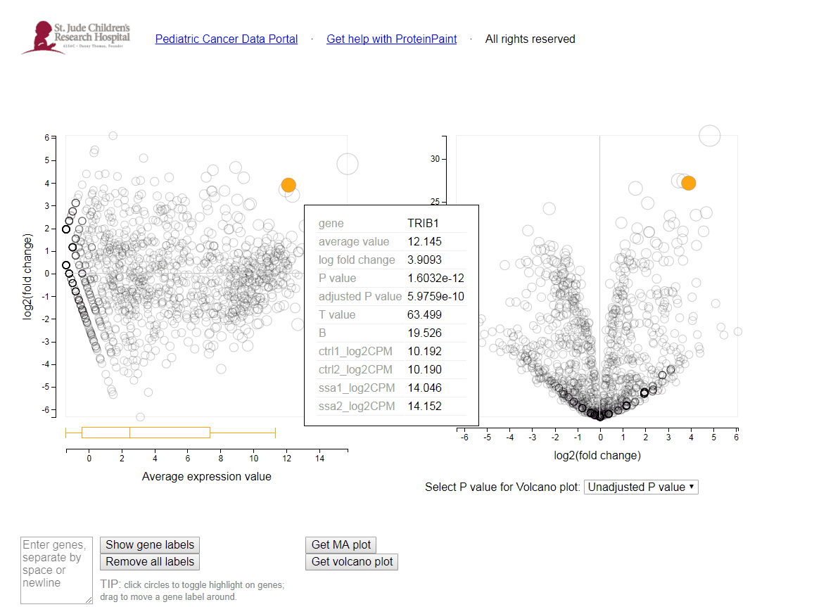
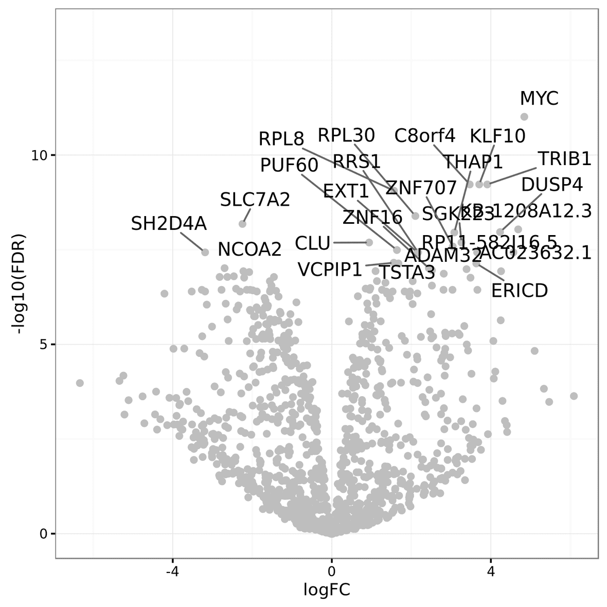
Within the root directory, there will be a viewer file for each valid comparison (limma.<contrast>.viewer). Simply select the file and press ‘Launch viewer’. A viewer will pop up showing both the MA plot and Volcano plot. By moving the mouse over a circle, the circle will highlight, and the corresponding feature on the other graph will also highlight. Additional information about the feature and its expression values will also be shown. One can also type in multiple feature identifiers in the provided text box. By pressing ‘Show gene labels’ all these features will be highlighted on the plots.

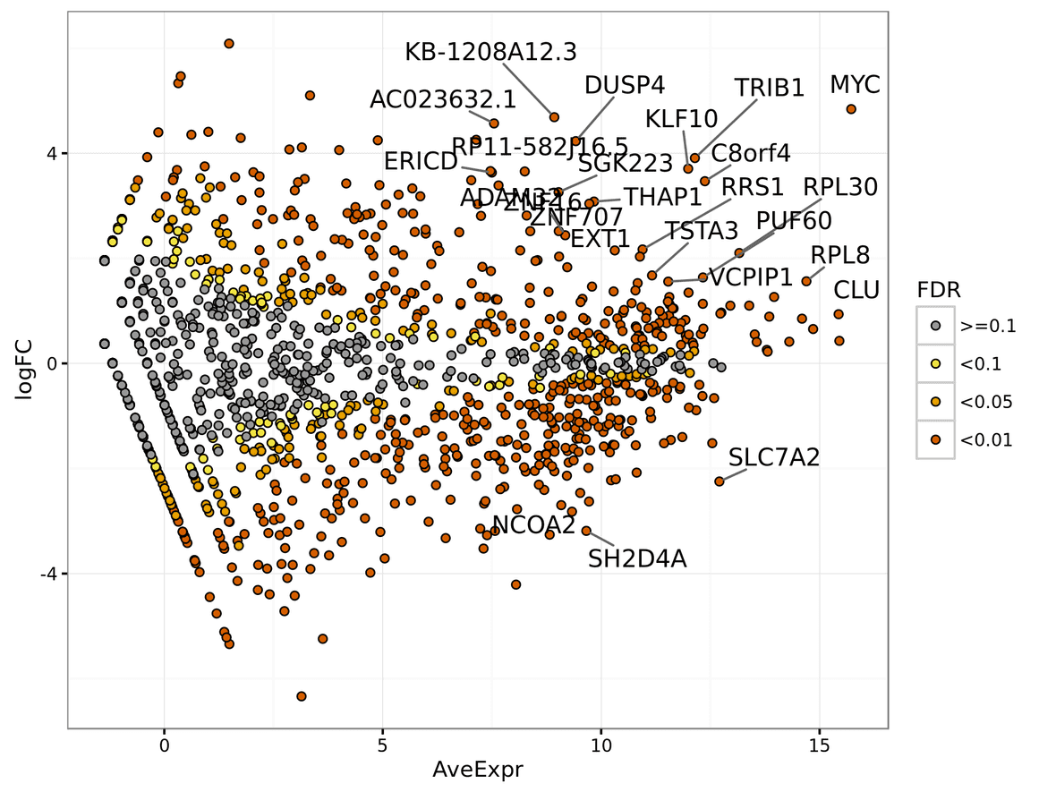
The MA plot shows the average expression of the feature on the X-axis, and Log2 fold change between condition/phenotype is on the Y-axis (if the name is for example MA_plot.condition2-condition1.png then the fold change would represent condition1 minus condition2). Each feature is represented by a circle. The top 20 feature (by p-value) are identified on the plot. The features are color coded by the chosen multiple testing correction method (False Discovery Rate (FDR) by default). An example MA plot can be seen below.

The volcano plot shows the Log2Fold change between the conditions on the X-axis, and the -Log10 of the multiple testing corrected P-value on the Y-axis.

Simple differential expression viewer

There will also be a viewer for the simple differential expression analysis in the root directory (simple_DE.<contrast>.viewer). The P-value for the results have all been set to 1, so the volcano plot will not be relevant. Static versions of the plots will be in the DIFFERENTIAL_EXPRESSION/ directory.

bigWig viewer

There will be a bigwig_viewer file if the option run_coverage was selected in either the FASTQ or BAM app. Select this file and then ‘Launch viewer’. A graph of coverage for the genome of all samples will be visible. This viewer can be found in the BIGWIG/ folder.

Combined count and FPKM files

HTSeq-count files are combined into a file called combined_counts.htseq.txt. If the counts were generated using “gene name” as the feature, then FPKM and FPKMlog2 files will also be combined into combined_counts.fpkm.txt and combined_counts.fpkm.log2.txt respectively. All of these will be found at the root of the output folder.

Secondary Results

Alignment statistics

alignment_statistics.txt shows alignment statistics for all samples. This file is a plain text tab-delimited file that can be opened in Excel or a text editor such as Notepad++. This file contains information on the total reads per sample, the percentage of duplicate reads and the percentage of mapped reads. An example of this file is below. This file will be in the STAR/ folder.

MA/Volcano Plots

In addition to viewing the MA and volcano plots through the visualization tool, static .pngs will be located in the DIFFERENTIAL_EXPRESSION/ directory.

Differential expression results

Other useful differential expression results will be created. This includes tabular output from the differential expression analysis. For each comparison with three or more samples per condition, results.limma.<contrast>.txt will be produced. results.simple_DE.<*contrast>.txt will be created for all comparisons, regardless of sample size. You can find a counts matrix normalized by Counts Per Million (CPM) in the file CPM_normalized_values.txt. All of these will be located in the DIFFERENTIAL_EXPRESSION/ directory.

GSEA.input.<contrast>.txt and GSEA.tStat.<contrast>.txt

These are input files that can be used for GSEA analysis. The tStat file is preferred for a more accurate analysis, but will not give a heatmap diagram. These files will be in the AUXILIARY/ directory.

Coverage results

bigWig files will be optionally generated (via the run_coverage option) for use in genome browsers (such as IGV http://software.broadinstitute.org/software/igv/). For each sample, multiple bigWig files may be found. For all types of sequencing strandedness, there will be bigWig files labeled, *.sortedcoverage_file.bed.bw where ’*’ is the sample name. For stranded data there will also be *.sortedPoscoverage_file.bed.bw and *.sortedNegcoverage_file.bed.bw which contains coverage information for the positive and negative strand of the genome. These files will be in the BIGWIG/ directory.

Quality Control Results (FastQC)

If FastQC was opted into (via the run_FastQC option), there will be a FASTQC/ directory. For each sample and read direction there will be an html file and a zip file (*.fastqc.html and *.fastqc.zip), containing results from FastQC. For the average user the html file is sufficient. This file can give some basic statistics on the quality of the data.

BAM alignment files

There may be up to 3 BAM files generated per sample that contain mapping information for all reads. The first is labeled *.Aligned.bam where ’*’ is the sample name. The BAM file is sorted by coordinates and will have duplicates marked (by default, but duplicate marking can be disabled with the mark_duplicates option). This is always generated and can be found in the STAR/ directory. If generate_name_sorted_BAM is enabled, then there will also be *.Aligned.name_sorted.bam in the STAR/ directory. The third file is optionally generated, *.Aligned.to_transcriptome.bam, and contains reads mapped to transcripts. This can be enabled with the generate_transcriptome_BAM option. If generated, these BAMs will be in the STAR/TRANSCRIPTOME/ directory.

Chimeric reads and junction files

Additional files created by STAR are provided. More information on these files can be found here. *.SJ.out.tab contain splice junction information. Fusion detection files are labeled *.Chimeric.out.bam and *.Chimeric.out.junction.

*.SJ.out.tab files will be in STAR/TABS and chimeric BAMs and chimeric junction files will be in the STAR/CHIMERIC/ directory.

FPKM and count files (per sample)

Per sample files containing FPKM and raw count values for each feature can be found in *.fpkm.txt, *.fpkm.log2.txt, and *.htseq_counts.txt where ’*’ is the sample name. Counts files will be in the HTSEQ/ directory, and FPKM files will be in HTSEQ/FPKM/.

Additional Outputs

Workflow parameters

WARDEN_parameters.json is the full list of parameters, including defaults, that were passed into this run of WARDEN. It can be found in the AUXILIARY/ folder.

Rerunning analysis

If you complete a WARDEN run from FASTQs or BAM files and wish to change some of the final differential expresssion parameters, we recommend you use the count files already generated as input to the “WARDEN [Counts]” app. This should save you sigfnificant amounts of time and money.

Similarly, if you started with FASTQs and wish to rerun with different parameters to HTSeq-Count, we recommend using the previously generated BAM files as input to the “WARDEN [BAM]” app.

BAM files and count files are output as soon as they are created (as opposed to only appearing after a successful analysis), so if you find WARDEN has failed for any reason at a later stage, you should be able to use the already output BAMs or count files to skip rerunning the stages which completed successfully.

You will need to update your “sample sheet” to include the new filenames if you wish to use this approach.

Frequently Asked Questions

Source code for the WARDEN apps can be found on our GitHub.

If you have any questions not covered here, feel free to reach out on our contact form.

Similar Topics

Running our Workflows
Working with our Data Overview Upload/Download Data (local)