RNA-Seq Expression Classification

Overview

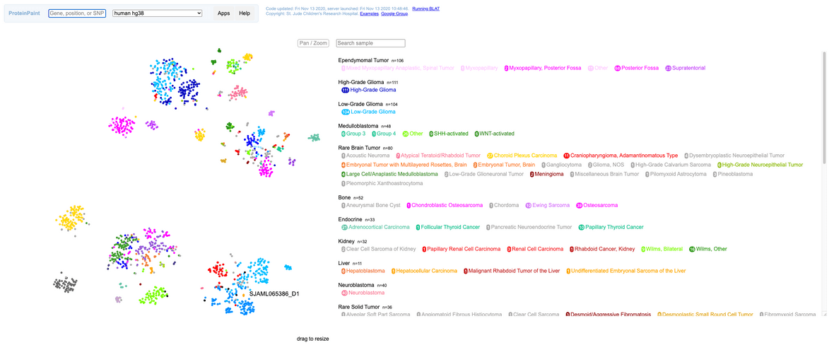
St. Jude Cloud provides functionality for generating RNA-Seq Expression Classification plots. This workflow allows plotting of RNA-Seq data by running through the St. Jude Cloud normalization pipeline. The generated count data is then compared to a reference set of data from a cohort of St. Jude samples and a plot is produced.

Requirements

• The RNA-Seq Expression Classification pipeline reference data uses sequencing data from fresh, frozen tissue samples. It has not been evaluated for use with sequencing data generated from formalin-fixed paraffin-embedded (FFPE) specimens.
• If running the count-based pipeline, alignment must be done against the GRCh38noalt reference. It should use parameters as specified in our RNA-Seq workflow to minimize any discrepancies caused by differing alignment specification.
• If running the count-based pipeline, feature counts should be generated with htseq-count as described in our RNA-Seq workflow. This pipeline uses Gencode v31 annotations.

Inputs

The input can be either of the two entries below, based on whether you want to start with a counts file or a BAM file.

Name	Description	Example
BAM file	Aligned reads file from human RNA-Seq	Sample.bam
Counts file	htseq-count output feature counts file from human RNA-Seq	Sample.counts.txt

Outputs

The RNA-Seq Expression Classification pipeline produces the following outputs:

Name	Description	Pipeline Version
Interactive expression plot (.html)	Visualization of RNA-Seq data	all
Aligned BAM (.bam)	BAM file produced by our RNA-Seq pipeline for the input samples.	Realignment
Feature read counts (.txt)	Read counts for the Gencode features.	Realignment
Gene list (.txt)	List of genes used in analysis (if a fixed list not specified)	all

Workflow Steps

1. [Only for realignment workflow] The aligned BAM is converted to FASTQ and is aligned to GRCh38_no_alt using standard STAR mapping.
2. [Only for realignment workflow] A feature count (.count.txt) file is produced for comparison to St. Jude Cloud reference data.
3. A visualization for genomic features is produced.

Mapping

We use the STAR aligner to rapidly map reads to the GRCh38 human reference genome.

Feature Counts

We use htseq-count to produce genomic feature counts.

Visualization

A t-Distributed Stochastic Neighbor Embedding (t-SNE) visualization is produced using Rtsne. You can find the t-SNE paper here.

Cost Estimation

Workflow Name	Per sample cost	Outliers
Realignment workflow	$3-10	$25
Feature read counts workflow	$0.30-0.40

Running the workflow

Getting Started

We provide two versions of the RNA-Seq Expression Classification workflow depending on desired input. The full workflow allows a user to upload a sample in BAM format. That sample will then be converted to FASTQ format, aligned with STAR two-pass alignment, and feature counts generated with htseq-count

To get started, you need to navigate to the RNA-Seq Expression Classification workflow page. You’ll need to click the “Start” button in the left hand pane. This creates a cloud workspace in DNAnexus with the same name as the workflow. After this, you will be able to upload your input files to that workspace.

Obtaining reference data

Reference feature count data is vended to the project folder along with the workflow. It can be found in the “counts” folder.

Reference data can also be retrieved through the Genomics Platform Data Browser

These must then be provided to the workflow through the reference_counts parameter. By default, all reference files will be used by the app, but this can be restricted to one of the three tumor types [Blood, Brain, Solid] through the app settings.

Running the workflow

Once you’ve uploaded data to your cloud workspace, click “Launch Tool” on the workflow’s landing page. A dropdown will present the different presets for running the workflow. Here, you can select whether you wish to start with a counts file or a BAM file. Once the workflow has been vended, copy the workflow to the project containing the reference data.

Uploading data

The RNA-Seq Expression Classification pipeline takes either a htseq-count count file or a GRCh38noalt aligned BAM from human RNA-Seq. You can upload your input file(s) through the command line. See Uploading Data from your Local Computer.

Once you have the dx toolkit, to upload a sample HTSeq count file sample.counts.txt to the inputs folder of the project-rnaseq cloud project, you could use the following command:

dx upload sample.counts.txt --destination "project-rnaseq:/inputs/"

Preparing input data

To run an input sample, certain properties need to be set on the file. These should be specified on the HTSeq count file for the counts-based pipeline or on the BAM file for the realignment-based workflow.

Property Name	Values
sample_name	should match filename up to first period (”.“)
library_type	PolyA or Total
read_length	integer, in bp
strandedness	Stranded-Forward, Stranded-Reverse, Unstranded
pairing	Paired-end or Single-end

Properties can be set at the job-level for all input files that do not have properties set. These function as defaults and will not override existing values on files. The options are limited to values in our reference cohort to ensure reliable results.

If a more granular control of covariates is needed, the input files can be annotated directly with properties. To input properties in DNAnexus, you can either use the web UI or the command line interface. Here, we provide a command line snippet to set properties on a file.

# you can run the following code snippet after filling in your values
# to successfully prepare the file.

file_id=<DNAnexus file ID> # file ID or file path
dx set_properties $file_id sample_name="<value>" # Should match the file name up to the first period character
dx set_properties $file_id strandedness="<value>" # Stranded-Forward, Stranded-Reverse, or Unstranded
dx set_properties $file_id library_type="<value>" # PolyA or Total
dx set_properties $file_id read_length="<value>" # Integer number of base pairs in reads (e.g. 101, 126)
dx set_properties $file_id pairing="<value>" # Paired-end or Single-end

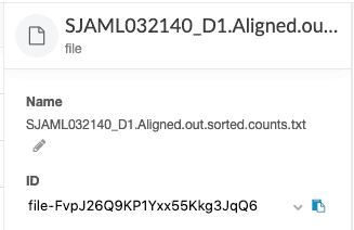
The file ID can be retrieved from the DNAnexus web interface. Click on the file of interest and the file ID is displayed in the sidebar.

Hooking up inputs

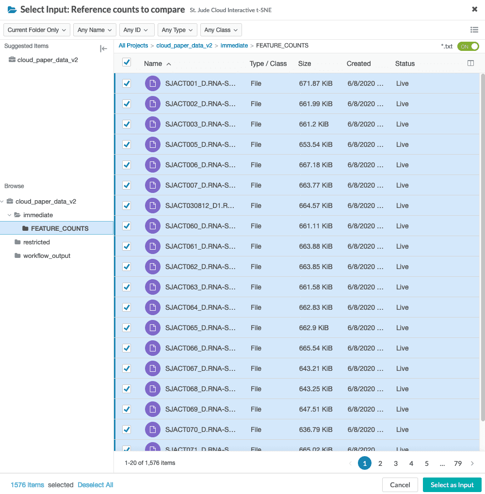
You will need to select reference counts files from your project. These can be specified in the reference counts data input.

When specifying the reference_counts, select all HTSeq count files in the reference dataset. For the St. Jude Cloud paper dataset, there are 1576 total files to select.

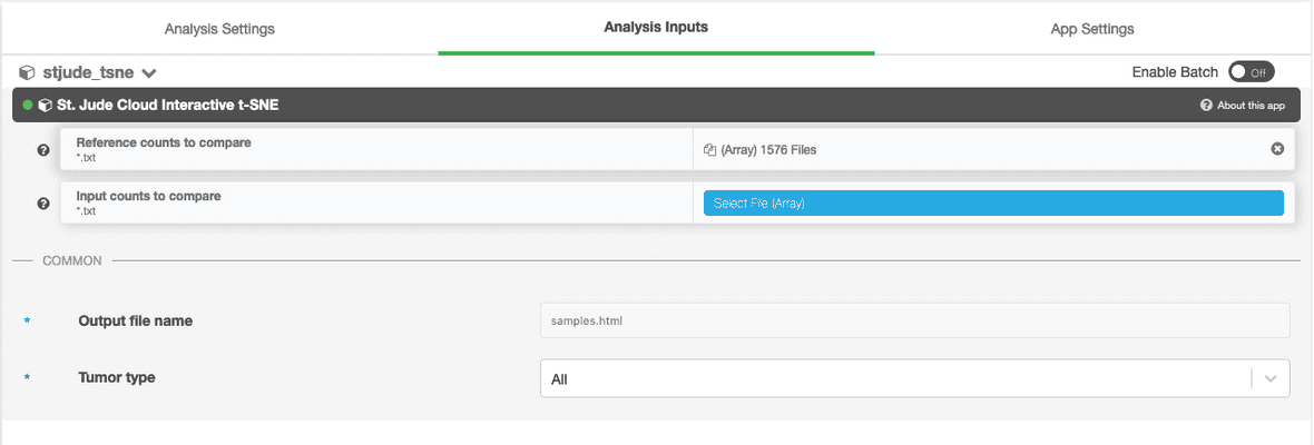
The UI will then display the number of selected reference files.

Next, you’ll need to hook up either the counts file or the BAM file you uploaded in the upload data section. In this example, we are using the counts-based version of the pipeline, so you can hook up the inputs by clicking on the input_counts slot and selecting the respective files. If you are using the realignment-based workflow, the process is similar with BAM input.

Additionally, a parameter selecting the tissue type to compare against can be selected. The available options are “Blood Cancer”, “Brain Tumor”, and “Solid Tumor”. Based on the selection, a reference collection of tumors of that type will be selected from St. Jude Cloud data and the input samples will be compared against this reference collection.

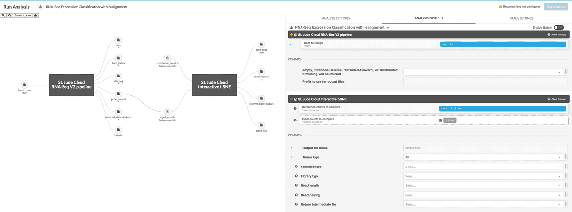
If running the realignment workflow, the input file should be specified as a BAM to realign. HTSeq will run on the realigned BAM and the result will be passed into the t-SNE app for plotting against the reference data. The reference data should be specified in the reference_counts parameter as an array of HTSeq count files. The BAM will be specified to the RNA-Seq V2 stage as input_bam. The BAM should have properties set as described above. These will automatically be applied to the new HTSeq count file.

Optional settings

An optional gene list can be specified as an input. This is a single column text file with gene names. If this option is specified, the list will override the default selection of the top 1000 most differentially expressed genes.

By default, all tumor types (blood, brain, and solid) will be included in the analysis. It is also possible to run each of the three types separately by selecting the appropriate tumor type.

The workflow supports both Fresh/Frozen and FFPE inputs. By default, only Fresh/Frozen samples from the reference cohort will be included. This setting can be changed to run only FFPE or Fresh/Frozen + FFPE samples.

It is also possible to return intermediate files from the workflow. If desired, ‘originalmatrix’ is the matrix of counts after covariates and additional metadata has been removed, ‘variancestabilized’ is the matrix after running varianceStabilizingTransformation, ‘batchcorrected’ is the matrix after ComBat batch correction, ‘tsneoutput’ is the matrix after Rtsne has been run and ‘matrix’ is the original file input to the R script for plotting.

The expression workflow can optionally include PDX samples from the reference cohort as well as a selection of PDX models from Dana Farber Cancer Insitute. The inclusion of PDX samples can facilitate selection of mouse models for followup functional experimentation.

Starting the workflow

Once your input files are hooked up, you should be able to start the workflow by clicking the “Run Analysis” button in the top right hand corner of the workflow dialog.

Monitoring run progress

Once you have started one or more RNA-Seq Expression Classification runs, you can safely close your browser and come back later to check the status of the jobs. To do this, navigate to the workflow’s landing page. Next, click “View Results” then select the “View Running Jobs” option. You will be redirected to the job monitoring page. Each job you kicked off gets one row in this table.

You can click the ”+” on any of the runs to check the status of individual steps of the RNA-Seq Expression Classification pipeline. Other information, such as time, cost of individual steps in the pipeline, and even viewing the job logs can accessed by clicking around the sub-items.

Interpreting Results

Once the resulting analysis job completes, an HTML plot of the results should be available. The plot is generated with the ProteinPaint library. The plot can be zoomed arbitrarily and group labels can be turned on/off for manual inspection. User input samples will be displayed in black marks with a label on the graph as well as an entry in the legend.

Batch effect corrections

When comparing numerous samples such as those included in this analysis, it is important to consider the variation in data created by obtaining from various sources and across time. Therefore the t-SNE visualization incorporates some batch effect corrections for the reference data. Currently we correct for batch effect based on strandedness of the RNA-Seq sample, library type, read pairing, and read length.

Batch Variable	Values
Library Type	PolyA or Total
Read Length	integer, in bp, e.g. 101, 126
Strandedness	Stranded-Forward, Stranded-Reverse, Unstranded
Pairing	Paired-end or Single-end

Known issues

There are a few known cautions with the RNA-Seq Expression Classification workflow.

Frequently asked questions

If you have any questions not covered here, feel free to reach out on our contact form.

Submit batch jobs on the command line

See How can I run an analysis workflow on multiple sample files at the same time?